The pathology is not the input.
It is the absence of normal form.
Parallax Pathology is a deterministic, training-free structural measurement system for H&E histology using the kernels. It learns what normal tissue looks like and measures as a fixed function how far any patch deviates from that. No labels required. No black box. Every output is traceable to a specific geometric property. It turns pathology from a classification problem into a measurable structural state space.
A measurement system that is built to show deviation from a structural norm, rather than a pattern to be approximated.
METHOD
A deterministic structural metric set for H&E Histology
Most computational pathology work trains CNNs or transformers to classify patches as "tumor vs. normal" etc. This instead asks: how is structure geometrically organized? It's more like a physics-style measurement system than a classification pipeline. The name "Parallax Pathology" hints at the philosophy, parallax is about viewing the same thing from multiple angles to get depth. Using a subset of colorectal cancer and healthy tissue as a case study:
58
deterministic scalar axes, v4 system
0
learned parameters
1,800
patches validated, CRC-VAL-HE-7K
91.5%
9-class accuracy, no training data
The instrument is built with:
Nine measurement layers, deterministic throughout
Each image is interrogated through nine measurement layers. The original six establish geometric and structural position. Three new layers added in v4 extend into texture and nuclear microstructure — carrying the system from 84.2% to 91.5% accuracy.
-
Nine geometric scalars on the confirmed edge field and baseline: centroid offset, void ratio, cohesion, spatial dispersion, packing density, peripheral pull, orientation coherence (θ), structural thickness.
-
Sixteen structural theories compared: Ω (cross-mask agreement), Γ (boundary permissiveness), Δᵣ (luminance–chromatic disagreement), Β (blind spot mass). The disagreement between theories is the primary output.
-
G1 centroid wander, G2 void topology and gland morphology, G3 contour curvature, G4 orientation entropy slope across scale, Structural Coherence Index.
-
How structural mass organizes relative to frame center versus its own center of gravity. Captures self-organizing versus frame-locked architecture.
-
LAB L* partitioned into shadow mass (dense nuclei), midtone mass (cytoplasm, stroma), and highlight mass (mucin, necrosis, open architecture). Strongest single-metric discriminator: F=604.
-
Class-conditional weighted distance from per-tissue structural norms. Returns nearest class, deviation scalar, and axis-level explanation. The memory layer — what the tissue is supposed to do.
-
Where Sobel fires but Canny does not: soft gradient transitions without hard boundaries. Captures diffuse infiltrates, early stromal remodeling, and blurry nuclear membranes. Most sensitive to structural transitions at tissue compartment boundaries.
-
Gray-Level Co-occurrence Matrix at fine scale (cellular, σ=2) and coarse scale (tissue, σ=16), on LAB L* and separately on Beer-Lambert hematoxylin and eosin channels. Chromatin texture and stromal fiber regularity as independent signals. Largest single gain: +5.1pp from tex_homogeneity_fine alone.
-
DoG blob detection on the hematoxylin channel counts nucleus-like structures and characterizes size distribution — density, mean radius, size irregularity — without cell segmentation. Adipose returns near-zero. Lymphocyte clusters return the system's highest densities.
Per-class Accuracy
ADI 99% | BACK 100% | DEB 93% | LYM 96.5% | MUC 97.5% | MUS 81.5% | NORM 95% | STR 74.5% | TUM 86.5%
From there, it can compare that tissue to a chosen reference, a typical example of that tissue type, and report how similar or different it is, and in what specific ways.
Instead of simply labeling tissue as tumor or normal, it can say: this area is less organized than expected, or the texture and structure do not match what we usually see here, and point to the exact features responsible. It behaves less like a predictive AI model and more like a measuring tool, giving a consistent, interpretable readout of tissue structure that can be used to compare samples, track changes, or understand where and how something is different.
The structural expectation layer
Memory of form
The instrument has no value without something to measure against. The Ω layer provides that: a reference distribution encoding what each tissue type is supposed to look like, and how tightly it must hold to that form. The system does not need a better metric, it needed a memory of what structure was supposed to be."
How the reference works
For each tissue class, the reference encodes three things: the mean structural position across 200 labeled patches, the per-axis variance (how tightly that class holds to each structural property), and the variance-inverse weight (which axes define that class versus which vary freely).
Low variance on an axis means the class is tightly defined there. Deviation on a tight axis contributes heavily to Ω. Deviation on an axis the class varies widely on barely registers.
Ω_c(x) = √( Σᵢ w_{c,i} · (xᵢ − μ_{c,i})² )
Where w_{c,i} = 1/(σ²_{c,i} + ε). Tighter classes penalize deviation more. Each tissue type defines its own structural rules.
| Class | Defining Axis | Weight | Meaning |
|---|---|---|---|
| LYM | θ (orientation) | 6,388 | Must be isotropic — any direction fails |
| NORM | θ (orientation) | 4,126 | Crypts produce omnidirectional gradients |
| TUM | θ (orientation) | 1.796 | Tumor lacks dominant direction |
| MUC | k_rv (void) | 635 | Mucus is defined by being mostly empty |
| ADI | k_rv (void) | 817 | Fat vacuoles are structurally empty |
| MUS | θ (orientation) | 166 | Fibers are directionally committed |
θ dominates 6 of 9 classes. Orientation coherence is the structural spine of the system — derived from the data, not designed in.
What Ω reveals
The gap between canonical and deviant
Across all seven clinical classes, canonical patches (bottom 10% Ω) and deviant patches (top 10% Ω) occupy completely non-overlapping ranges. The separation is not designed — it emerges from the variance-weighted distance structure.
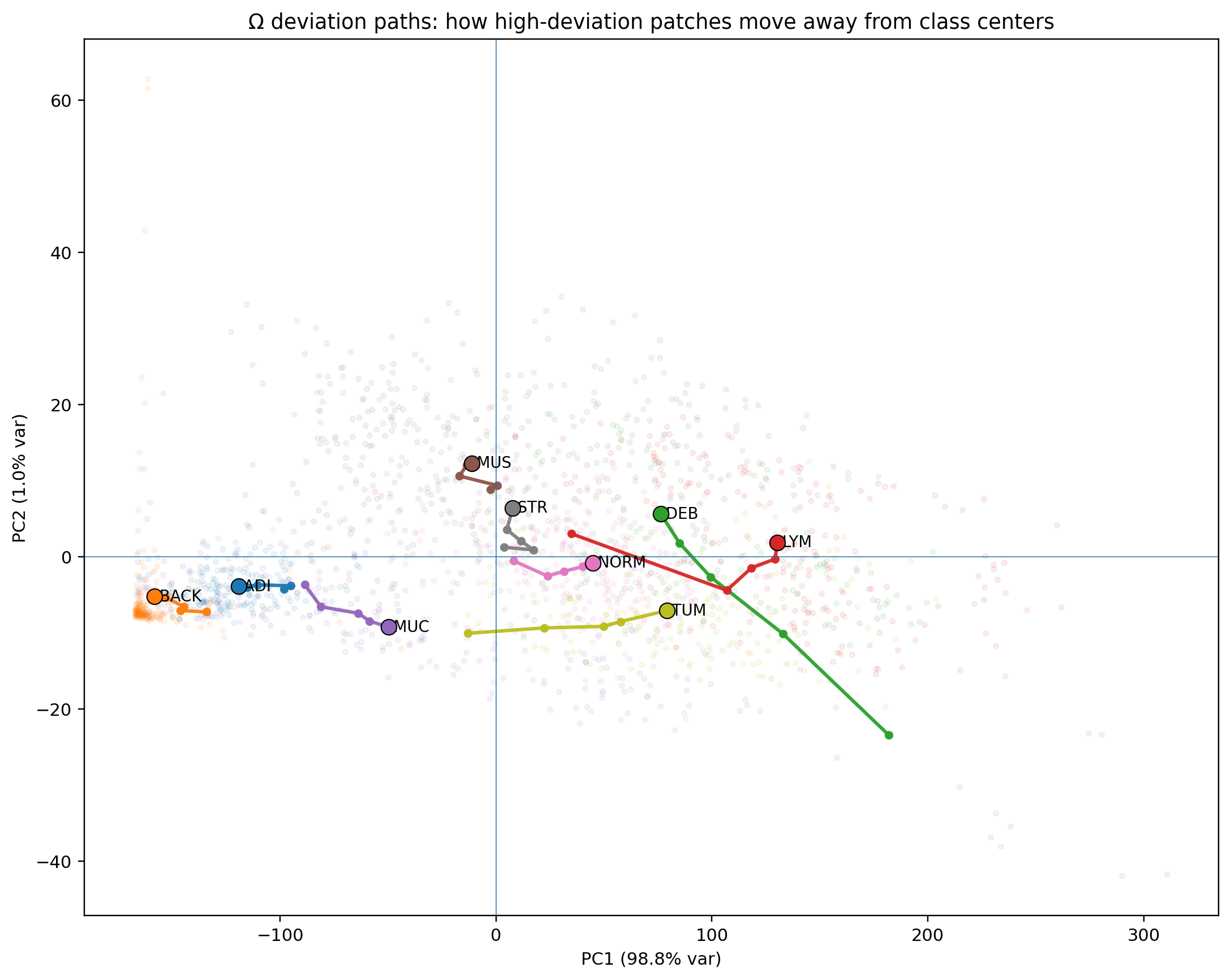
| Class | Canonical Range | Deviant Range | Primary Failure | Structural Drift |
|---|---|---|---|---|
| ADI | 0.35 – 0.76 | 4.64 – 7.63 | Δᵣ ↑ | → MUC |
| LYM | 0.81 – 1.41 | 3.06 – 6.02 | k_rv ↑ | → STR |
| MUC | 0.82 – 1.22 | 3.72 – 4.91 | k_rv ↓ | → ADI |
| MUS | 0.60 – 1.01 | 3.79 – 4.67 | θ ↓ | → STR |
| NORM | 0.56 – 0.99 | 3.96 – 4.72 | Δᵣ ↑ | → STR / MUC |
| STR | 0.51 – 1.25 | 3.83 – 4.59 | Δᵣ ↑ | → MUC |
| TUM | 0.32 – 0.78 | 3.99 – 5.71 | Δᵣ ↑ | → STR |
Drift direction = most common nearest class among top 10% deviant patches. Visual inspection confirmed all seven classes.
Key finding — TUM
When tumor stops being tumor
The most clinically significant result in the validation: deviant tumor patches do not fail randomly. They fail in two geometrically distinct ways — and each way maps to a recognized biological phenomenon, detected without a single labeled example of either.
Failure mode 01
Density loss
Highlight mass jumps from 0.229 (canonical) to 0.54–0.61. Gamma spikes to 0.60–0.67. The tumor field opens. Dense epithelial sheets give way to optically permissive space.
Geometric signature of mucinous differentiation, intratumoral necrosis, or poorly cohesive growth — recognized histological subtypes with distinct biological behavior.
highlight ↑ +0.220
gamma ↑ +0.205
midtone ↓ −0.236
Failure mode 02
Directional acquisition
θ jumps to 0.12–0.13 — nearly five times the canonical TUM mean of 0.024. These patches have acquired directional structure that tumor normally lacks entirely.
Geometric signature of desmoplastic reaction: host stromal fibrosis within the tumor field, the fibrous matrix of the tumor microenvironment displacing the epithelial architecture. Associated with invasion and poor outcomes.
θ ↑ ×5 vs canonical
Δᵣ ↑ +0.023
Both phenomena were detected without training on mucinous carcinoma, necrosis, or desmoplastic reaction. The system identified them through geometry alone, density loss registers as a highlight mass and gamma shift; desmoplasia registers as a θ acquisition.
The explainability advantage
The why is built into the measurement
Standard deep learning produces confident predictions without structural explanation. Every output from this system is traceable to a specific geometric relationship between specific channels.
Deep learning output
class: TUM
confidence: 94.3%
explanation: —
Parallax output
nearest class: TUM
Ω distance: 4.71
primary axis: highlight_mass ↑
contribution: 46.2%
reading: cellular density failing
The explanation is not post-hoc attribution. It is the measurement itself. A pathologist can read the axis output, recognize the structural property it refers to, and evaluate whether the measurement corresponds to what they see in the image.
Applications
Where this system has teeth
This is not a replacement for deep learning. It is a complementary instrument that does what deep learning does not — deterministic structural measurement, label-agnostic positioning, and deviation detection without pathological training examples.
◈
Rare disease and low-data settings
Building a reference requires only normal tissue examples — not labeled pathological ones. Normal tissue is almost always more available than labeled rare-disease datasets. A small lab can build a structural normal reference and immediately begin quantifying deviation in their cases of interest.
◉
Interpretability layer for deep models
The 60 deterministic outputs per patch form a structured, biologically meaningful feature representation. Concatenated with a foundation model's embedding, or used to explain predictions, the structural vector adds interpretable geometry to high-accuracy learned representations.
⊚
Continuous structural metrics
Ω is a continuous scalar — a distance, not a class. Multiple measurements over time produce a structural trajectory. Tissue drifting toward a pathological state shows increasing Ω before a defined diagnosis is possible. This is underexplored in computational pathology.
◎
Out-of-distribution detection
Deep models classify confidently within their training distribution — and fail confidently outside it. This system has no training distribution. High Ω on an unseen tissue type means "this does not fit any known structural regime" — the correct output, not a misclassification.
⊗
Dysplasia as measurement
Clinical pathology describes dysplasia as disordered growth and judges it qualitatively. Structural dissonance — the axis-decomposed Ω score — offers a geometric operationalization of the same property, with known inter-observer variability replaced by a deterministic scalar.
⊕
Library of normals
The reference architecture generalizes across tissue types. Build a normal reference for breast, skin, or kidney — and pathological cases surface as deviations from that reference, without labeled examples of the pathology itself. One architecture, any tissue.
Research paper
Parallax Pathology:
A Deterministic Structural Expectation Framework
We introduce Parallax Pathology, a deterministic, training-free structural measurement system for H&E stained histology images.
On CRC-VAL-HE-7K (1,800 Macenko-normalized 224px patches, 9 tissue classes), the system achieves 91.5% nine-class linear accuracy without any training, and produces visually confirmed structural separation between canonical and deviant patches across all seven clinical classes. A key finding is that deviant tumor patches stratify into two geometrically distinct failure modes corresponding to mucinous/necrotic differentiation and desmoplastic stromal reaction — detected through geometry alone.
Get the instrument
Everything needed to run it
Two notebooks, one reference file, one enriched dataset. Deterministic — the same image produces the same output on every run.
Single-image notebook
Full visual output — mask grid, kernel primitives bar chart, structural complexity curves, radial compliance, tonal structure, structural position Ω. Drop in any H&E image and run.
Batch runner
Process directories of images, output a master CSV with all 60 metrics and Ω distances for every patch. Includes the Ω Reference Builder — point it at a labeled corpus to generate your own reference.
Ω reference — colorectal
Structural expectation reference built from CRC-VAL-HE-7K. Per-class mean, variance, and weight vectors for 6 metrics across 9 tissue types. Drop into /content/ and Ω fires automatically.
Validation dataset
All 1,800 CRC-VAL-HE-7K patches enriched with the full 60-metric output plus Ω distances to all 9 reference classes. All tables and figures in the paper are reproducible from this file alone.