The pathology is
the absence
of normal form.
Parallax Pathology is a deterministic, training-free structural measurement system for H&E histology using the kernels. A deterministic, training-free structural measurement system for H&E histology. Sixteen structural theories. Fifty-eight axes. No labeled pathological examples required.. No black box. Every output is traceable to a specific geometric property. It turns pathology from a classification problem into a measurable structural state space.
Rather than learning what pathology looks like, the system learns what structural norm looks like and measures deviation from that norm.
Benchmark CRC-VAL-HE-7K · 1,800 patches · 9 tissue classes
Accuracy 91.5% nine-class linear accuracy · zero training
External validation EBHI-SEG dysplasia grading · GTEx cross-dataset · TCGA-COAD survival
METHOD
A deterministic structural metric set for H&E Histology
Most computational pathology work trains CNNs or transformers to classify patches as "tumor vs. normal" etc. This works in collaboration, but asks: how is structure geometrically organized? It's more like a physics-style measurement system than a classification pipeline. The name "Parallax Pathology" hints at the philosophy, parallax is about viewing the same thing from multiple angles to get depth. Using a subset of colorectal cancer and healthy tissue as a case study:
16.3pp
EMERGENCE GAP
Best single layer scores 75.2%. Full 58-axis system: 91.5%. The combination is genuinely greater than any component.
0
TRAINED PARAMETERS
Every output is traceable to a specific geometric relationship. The explanation is the measurement, not post-hoc attribution
r = 0.72
DYSPLASIA GRADE CORRELATION
Spearman ρ on EBHI-SEG (n=920). Structural geometry tracks continuous biological progression never shown.
91.5%
9-CLASS ACCURACY
CRC-VAL-HE-7K, 5 fold cross-validation. No training. 58 deterministic aces vs. the benchmark.
HR=1.872
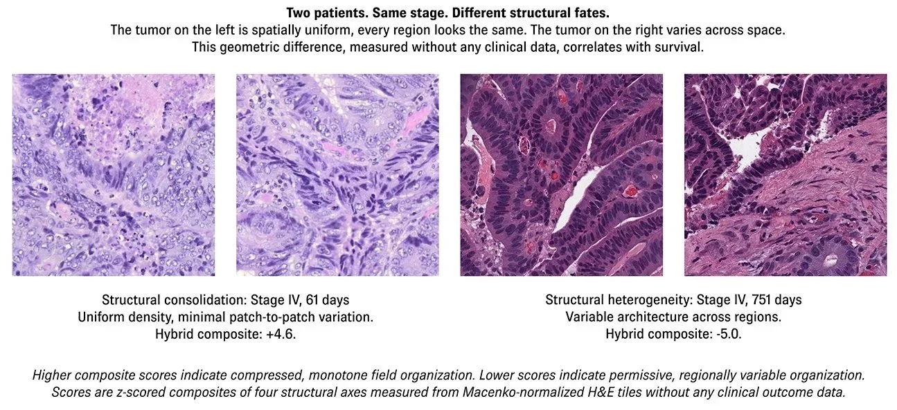
STRUCTURE ACROSS SPACE, NOT AVERAGES
Disease-specific survival hazard ratio from a normalized hybrid composite of four geometric axes — void permissiveness, luminance-chromatic disagreement, and intra-tumor structural variability. No outcome training. No molecular data. Stage-adjusted.
3.3x mortality difference, low vs. high tertile. p=0.0002, DSS. C-index: 0.808.
01 — The Core Inversion
A different question requires a different instrument.
Standard approach
Train on labeled pathology. Learn what disease looks like.
Foundation models trained on millions of labeled patches achieve 95–99% accuracy on standard benchmarks. Their predictions are confident and often correct. But they require large labeled datasets of pathological examples — and they cannot explain which geometric properties drove the prediction. They produce a verdict, not a reading.
Parallax Pathology approach
Learn what normal looks like. Measure the departure.
The system encodes the structural laws of normal tissue — what orientation coherence, void topology, boundary permissiveness, and tonal distribution look like when tissue is doing what tissue of its type does. Deviation from those laws is the signal. A rare disease the system has never seen will register as structurally distant from all known normals. That is not a misclassification. It is the correct output.
01. The Frame — invariant
Fixed axes
Six structural axes — Δᵣ, θ, Γ, k_rv, highlight_mass, midtone_mass — plus 52 additional geometric, texture, and microstructure features. The frame defines how structure is measured, not what structure should be. It does not change between a colorectal biopsy and a breast biopsy.
The thermometer.
02. Ω — structural deviation
The reading
Ω(x) = √( Σᵢ wᵢ · (xᵢ − μᵢ)² ) where wᵢ = 1/variance. A continuous scalar measuring how far a patch sits from the structural expectation of a chosen reference class. Decomposed by axis — the source of deviation is always named.
Low Ω = tissue doing what that tissue does.
High Ω = failing to be itself.
03. The Memory — inserted
Swappable reference
A reference distribution built from representative normal examples of any tissue type. The memory is not part of the instrument — it is context provided to the instrument. Swap the memory for breast, kidney, or skin tissue. The frame stays. This is the Library of Normals architecture.
The reference temperature.
02 — The System
Nine layers. Fifty-eight axes. All deterministic.
-
Nine geometric scalars on the confirmed edge field and luminance baseline. Centroid, void ratio, mass concentration, packing density, orientation coherence, structural thickness. The same compositional primitives that describe painting structure describe tissue architecture.
-
Sixteen independent structural theories applied simultaneously: VTL baseline, LMS cone channels, opponent channels, color-deficiency ablations, H&E deconvolution, Canny-derived masks. Four coherence scores from their pattern of agreement and disagreement.
-
Centroid wander across scale (G1), void topology (G2), contour curvature variance (G3), orientation entropy slope over log(σ) (G4), and Structural Coherence Index. G4 is the strongest single axis for dysplasia progression detection.
-
How structural mass organizes relative to frame center versus its own center of gravity. Captures self-organizing versus frame-locked architecture.
-
LAB L* partitioned into shadow mass (dense nuclei), midtone mass (cytoplasm, stroma), and highlight mass (mucin, necrosis, open architecture). Strongest single-metric discriminator: F=604.
-
The deviation layer. Reference encodes per-class mean and variance-inverse weights. Ω computed for all reference classes simultaneously. Returns nearest class, own-class distance, top driving axis, and full per-class distance profile. Label-agnostic by design.
-
Surfaces the Sobel-minus-Canny residual — soft gradient regions that lack hard boundaries. Captures diffuse infiltrates, early stromal remodeling, nuclear membranes in transition. gap_rv (void ratio of the gap field) is a progression marker.
-
Gray-Level Co-occurrence Matrix at fine (cellular) and coarse (tissue) scales on luminance channel, plus separately on Beer-Lambert deconvolved hematoxylin and eosin channels. tex_homogeneity_fine produced the single largest accuracy gain: +5.1pp.
-
Difference-of-Gaussians (DoG Nuclear) detector on the hematoxylin channel. Nuclear density, mean size, and size coefficient of variation — a nuclear pleomorphism index — without requiring individual cell segmentation. Adipose correctly returns near-zero blob counts.
03 — Validation
Three datasets. Three different questions.
EBHI-SEG · Dysplasia Grading
Tracks a continuous biological progression never trained on.
Six-class dysplasia grading from Normal through Adenocarcinoma (n=920, 224px PNG). Adjacent classes overlap structurally by nature — this is not a classification problem, it is a measurement problem. 84.3% of predictions are correct or within one adjacent grade step. The system correctly places serrated adenoma structurally distinct from conventional low-grade neoplasia, consistent with its separate BRAF molecular pathway.
Spearman ρ (grade vs. predicted) 0.716
Correct + adjacent 84.3%
Progression axes p < 10⁻¹⁸ 11
Ridge R² (grade variance explained)
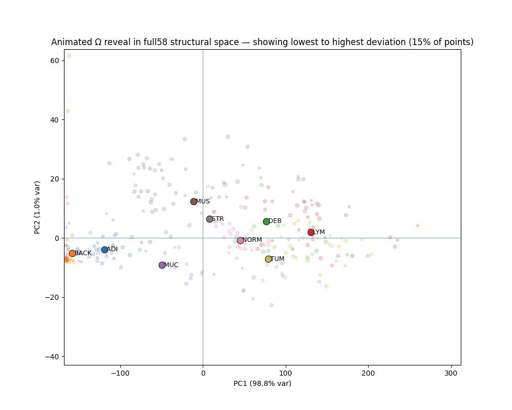
CRC-VAL-HE-7K · Tissue Classification
Tissue types occupy geometrically distinct, linearly separable regions.
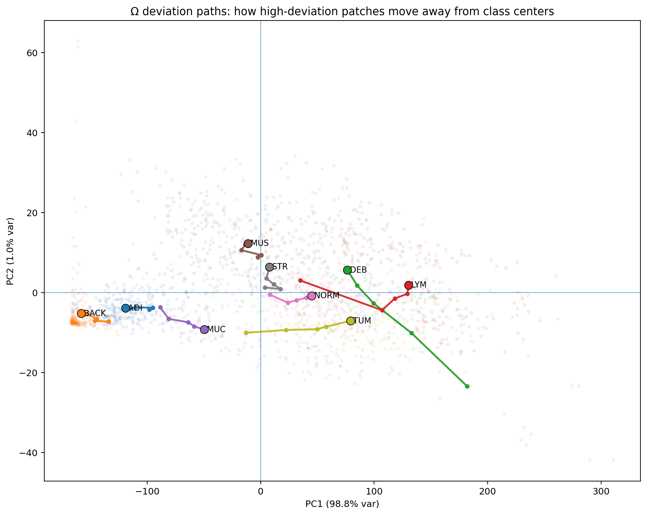
1,800 Macenko-normalized 224px patches across 9 classes. Every tissue class shows visually confirmed canonical/deviant separation. Deviant TUM patches stratify into two geometrically distinct failure modes corresponding to mucinous differentiation and desmoplastic reaction — detected from geometry alone, without pathological labels.
Overall accuracy 91.5%
ADI / BACK 99% / 100%
Emergence gap 16.3pp
Trained parameters 0
GTEx · Cross-Dataset Fixation
The frame is universal. The memory is not, and shouldn’t be.
Three independent GTEx whole slide images (PAXgene fixation — different preparation method from the formalin-fixed CRC-VAL data). Structural centers emerge independently within each donor without labels. Within-set Ω distributions (mean 2.09–2.26) are consistent with CRC-VAL results. A preparation chemistry finding: Δᵣ inverts its role in the deviation field between fixation methods, correctly detecting a real property of the tissue-chemistry interaction.
Donors tested 3 independent
Mean Ω convergence 2.09–2.26
Cross-preparation stable axes k_rv, θ
Labels required 0
TUM Deviant Analysis · Failure Mode 1
Density Loss
highlight_mass jumps from canonical mean 0.229 to 0.54–0.61. The tumor field opens, cellular density gives way to optically permissive space. Geometric signature corresponds to mucinous differentiation, intratumoral necrosis, or poorly cohesive growth — detected without training on either.
highlight_mass (Δ) +0.22 ↑ field opening
Γ — boundary permissiveness +0.21 ↑ losing definition
midtone_mass (Δ) −0.24 ↓ core density failing
TUM Deviant Analysis · Failure Mode 2
Directional Acquisition
θ jumps to 0.12–0.13, nearly five times the canonical TUM mean of 0.024. These patches have acquired directional structure that the tumor normally lacks. Geometric signature corresponds to desmoplastic reaction: host stromal fibrosis within the tumor field.
θ — orientation coherence 5× canonical → desmoplastic
Δᵣ — luminance-chromatic +0.02 ↑ structural tension
Drift destination → STR (stroma, 80%)
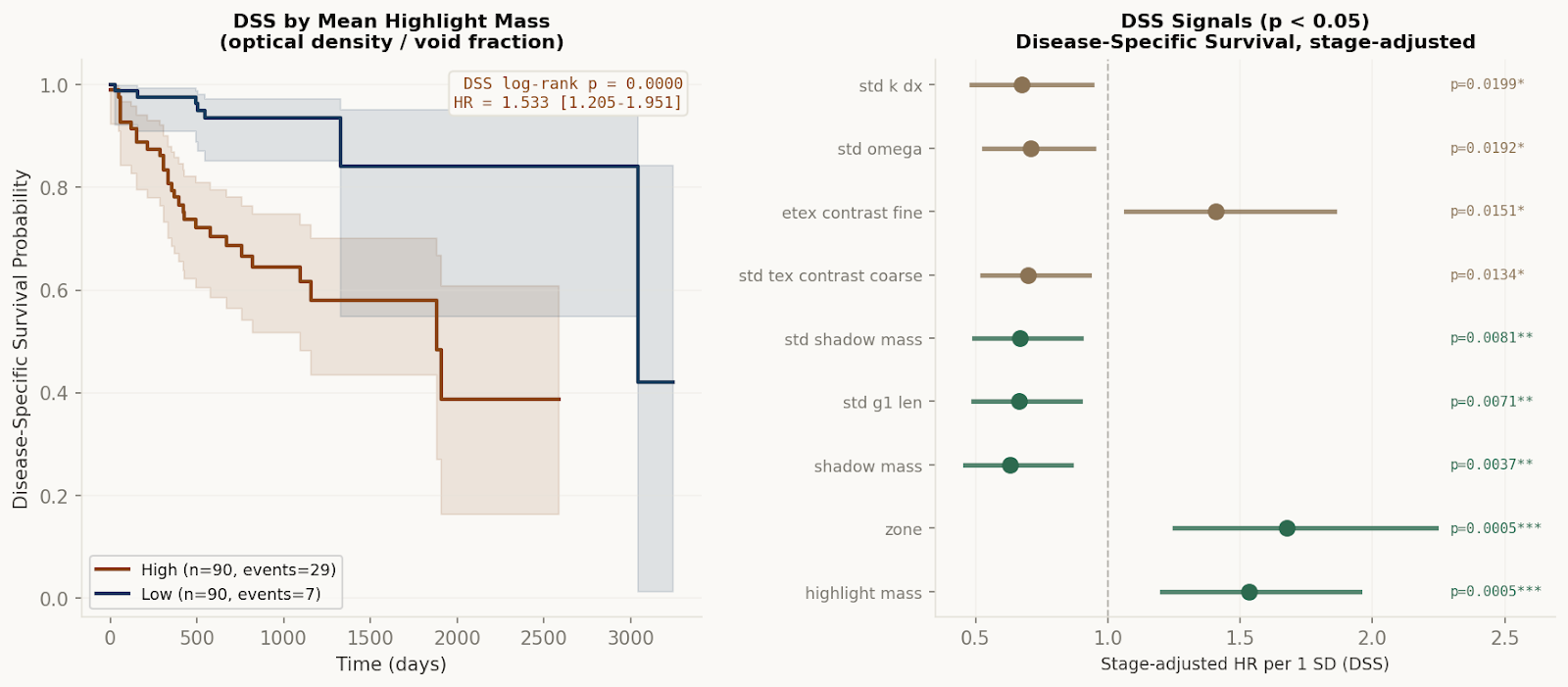
The honest null, and what it revealed.
TCGA-COAD survival analysis (n=180 colorectal patients, 47 OS events, 36 DSS events). The pre-specified primary hypothesis — that mean structural deviation (Ω) predicts overall survival — was not supported. HR=0.766, p=0.132. This result is reported directly, not minimized. It is also the most important methodological finding: the average tumor state does not predict outcome. What predicts outcome is how structural states are distributed across tumor regions.
After Macenko stain normalization removed preparation-chemistry variation across TCGA acquisition sites, eleven structural axes showed directionally consistent significant associations with both overall and disease-specific survival. They organized into two coherent field states: tumors that retain spatial openness, void permissiveness, and regional variability do better; tumors that have settled into spatial compression, high packing density, and structural monotony do worse. A normalized hybrid composite capturing this distinction stratifies patients with observed OS mortality of 13.3%, 26.7%, and 38.3% across tertiles. Disease-specific survival hazard ratio: 1.872 [1.343–2.608], p=0.0002 — without any outcome training. Concordance index on DSS: 0.808.
3.3× mortality difference,
low vs. high composite tertile HR=1.872 DSS,
no outcome training p=0.132 primary hypothesis, honestly null
04 — The frontier is explicit.
Where this system has teeth
04 — The frontier is explicit.
A foundation model answers
What is this tissue?
Confident categorical prediction. 95–99% accuracy on standard benchmarks. Optimized for classification. Requires large labeled datasets of pathological examples. Cannot explain which geometric properties drove the confidence. The gap in accuracy between deep learning and Parallax Pathology is real and expected — it reflects genuinely non-geometric information that no hand-designed feature encodes. This gap is not hidden. It is documented explicitly in the paper.
Parallax Pathology answers
How far is this tissue from what tissue of this type is supposed to do structurally, and which geometric axis is failing?
Continuous deviation scalar. Axis-level explanation built into the measurement itself. No training on pathological examples. No training distribution — high Ω on an unseen tissue type means the geometry does not fit any known structural regime. That is not a misclassification. It is the correct output. Rare diseases surface as high-deviation from all normals.
Parallax Pathology is a deterministic measurement framework that quantifies how tissue structure deviates from a learned reference of normal morphology. Rather than learning disease categories, it defines a structural baseline and measures displacement from it. Results do not establish a clinical biomarker, but demonstrate that explicit geometric measurements of tissue organization can capture reproducible and interpretable structure beyond standard learned representations.
-
Building a reference requires only normal tissue examples — not labeled pathological ones. Normal tissue is almost always more available than labeled rare-disease datasets. A small lab can build a structural normal reference and immediately begin quantifying deviation in their cases of interest.
-
The 60 deterministic outputs per patch form a structured, biologically meaningful feature representation. Concatenated with a foundation model's embedding, or used to explain predictions, the structural vector adds interpretable geometry to high-accuracy learned representations.
-
Deep models classify confidently within their training distribution — and fail confidently outside it. This system has no training distribution. High Ω on an unseen tissue type means "this does not fit any known structural regime" — the correct output, not a misclassification.
Applications
This is not a replacement for deep learning. It is a complementary instrument that does what deep learning does not — deterministic structural measurement, label-agnostic positioning, and deviation detection without pathological training examples.
-
Ω is a continuous scalar — a distance, not a class. Multiple measurements over time produce a structural trajectory. Tissue drifting toward a pathological state shows increasing Ω before a defined diagnosis is possible. This is underexplored in computational pathology.
-
Clinical pathology describes dysplasia as disordered growth and judges it qualitatively. Structural dissonance — the axis-decomposed Ω score — offers a geometric operationalization of the same property, with known inter-observer variability replaced by a deterministic scalar.
-
The reference architecture generalizes across tissue types. Build a normal reference for breast, skin, or kidney — and pathological cases surface as deviations from that reference, without labeled examples of the pathology itself. One architecture, any tissue.
05 — Broader Framework
Geometry as a perceptual instrument.
Origin
The Visual Thinking Lens
Parallax Pathology extends the Visual Thinking Lens (VTL), a geometric kernel originally developed for compositional analysis of AI-generated images and visual art. The same field-agnostic primitives — centroid, void ratio, orientation coherence, spatial dispersion — that describe compositional structure in paintings describe tissue architecture in H&E sections. The frame is universal. The application is not.
Principle
Finding the ceiling of what geometry can see
The system is explicitly not competing with foundation models. It is asking a different question with a different instrument: how far can deterministic geometric measurement go? At 91.5% nine-class accuracy without any training, the answer is: further than expected. The 16.3pp emergence gap confirms that the structural layers encode genuinely complementary information — not redundant signals averaging together, but a genuinely new capability from their combination.